The Kelly Criterion

The Kelly criterion is used to allocate a fraction of capital to a particular investment, given a payoff amount and an estimate of success, such that the growth rate of capital is maximized while simultaneously avoiding bankruptcy.

This method can be used to systematically allocate assets over a variety of investments with heterogenous risks. It is also It has been mentioned that some investment managers use the Kelly Criterion or variants of it to allocate their capital across their investment portfolios, although it is not clear if this has led more success than those that have not.

In this article, we will review how to compute the criterion by replicating the results of a research paper. We will then apply it to another use case involving stock options.

Kelly Criterion Overview

Intuitively, the Kelly criterion attempts to maximize the logarithm of expected return. In the case of continuous returns, we can express expected return as \[ G(f) = \int \log(1+fs) F(s) ds, \] where $F(s)$ is the probability of observing a return of $s$ and $\log(1+fs)$ is the logarithm of the growth rate. $f^*$ is the fraction of capital to invest that maximizes growth while avoiding bankruptcy and can be computed using numerical integration and optimization methods.

In the discrete case, the growth rate is expressed as \[ G(f) = E \log\frac{X_n}{X_0} = p\log(1+bf) - q\log(1-f) \] and \[ f^* = \frac{bp-q}{b} \].

Values of $-1 \le f < 0$, can be interpreted as taking a fractional short position. While $f \le -1$ indicates a short position using leverage. The opposite is true for positive intervals. $0 \le f < 1$ correspond to fractional long positions and $f > 1$ indicate long positions using leverage. Using these values to gauge investment size ensure that the investor maximizes growth while avoiding bankruptcy in the long run.

An Example

In Rotando's and Thorp's paper, The Kelly Criterion and the Stock Market, the authors compute $f^*$ for investing in the S&P 500. They begin by first collecting historical annual return data from 1926 to 1984 and fit the results to a Gaussian distribution. They estimate $\hat{\mu}$ as 0.058 and $\hat{\sigma}$ as 0.216.

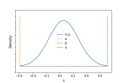
They go on to modify the distribution to satisfy their own view of the return structure of the stocks by clipping the tails and adding two constants, $\alpha$ and $h$, to make the optimization produce relevant results. The left tail boundary, denoted as $A$, is -0.59 and the right tail boundary, denoted as $B$, is 0.706. $\alpha=0.2183$ and $h= \frac{1 - 0.997006378}{B - A}$

The modified Gaussian distribution is shown below with the boundaries and values of $A,B$ and $h$ marked as dashed lines.

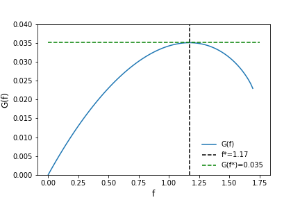
Now using the modified Gaussian probability distribution for expected returns as $F(s)$, the authors compute $f*$ by maximizing $G(f)$ with respect to $f$. \[ G(f) = \int_A^B \log(1 + fs)F(s)ds \] They obtain a value of $f^*=1.17$ and a value for $G(f*) = 0.0350444711$. Visually, we can inspect the function over valid values of $f$, which, per the paper, lie on $0 \ge f \le -1/A$. The figure below clearly shows $G(f)$ peaking at the saddle point, $f^*$.

Using scipy's numerical integration and optimization routines, we can obtain the same result. The code, using the constants reported in the paper, is shown below. After optimizing the function, scipy returns a result for $f = 1.17$. Using this value of $f$, $G$ is then calculated as \[ G(f) = \int_A^B \log(1+1.17s) F(s) ds = 0.0350444708, \] nearly identical the result in the paper.

import numpy as np
import scipy.stats
from scipy.optimize import minimize

def kelly(f):
    A = -0.59
    B = 0.706
    mu = 0.058
    alpha = 0.2183
    h = (1 - 0.997006378) / (B - A)
    rv = scipy.stats.norm(mu, alpha)
    result, error = quad(lambda i: np.log(1+f*i)*(h + rv.pdf(i)), A, B)
    return -result

minimize(kelly, 0)
  fun: -0.03504448268515331
  hess_inv: array([[15.89634431]])
  jac: array([-3.95812094e-06])
  message: 'Optimization terminated successfully.'
  nfev: 21
  nit: 5
  njev: 7
  status: 0
  success: True
   x: array([1.17055956])

Exploring Further

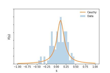
Now that we have an understanding of the criterion and how to compute f, let's apply it to other investments and examine how the criteria changes with a different $F(s)$. To do this, we will replicate the example above using annual return data for the S&P 500 from 1928 to 2020 and changing $F(s)$ from a Gaussian to a Cauchy. The figure below plots return data as well as the estimated $F(s)$ for the Cauchy over the domain $(-1,1)$.

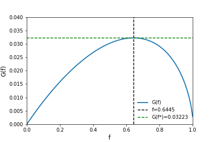
To maximize $G(f)$ and obtain meaningful results, $\int_{-1}^1F(s)ds$ needs to integrate to 1. Therefore, as in the paper, we need to add the density outside the lower and upper tail back in such that $h + \int_{-1}^1F(s)ds = 1$. The density, $h=0.07388$. Maximizing $G(f)$ as before, we find the optimal value of $f \in (0, -1/A)$ equal to $f^*=0.64450548$ and $G(f^*) = 0.03223$. The figure below plots $G(f)$ along with $f^*$.

Clearly, the choice of $F(s)$ plays a large part in choosing $f^*$. A Cauchy choice leads to an investment size that is 45% smaller compared with the Gaussian choice presented in the paper. In addition to this, one should also consider what long run return really means. In the paper and prior articles, empirical loss probabilities are presented that show in the first 5 years of an investment, losing material amounts of an investment have occurred relatively frequently. This has led many users of the method to think of $f^*$ as an upper bound on the maximum amount of investment one should consider making.

Conclusions

The Kelly Criterion has a rich history and has been incorporated into numerous investment strategies and decisioning processes. For more on this, the text The Kelly Capital Growth Investment Criterion presents a comprehensive survey of the research and thinking that has developed since the original work was shared.