Empirical Analysis Of Modern Portfolio Theory
What can over five million monthly stock returns tell us about modern portfolio theory (MPT) and the capital asset pricing model (CAPM)? Mainly, that stocks do not have the properties necessary to support the conclusions of these theories. In this article, I present a cursory overview of MPT and the CAPM. Then I perform a simple statistical analysis that clearly shows stock returns do not completely satisfy the assumptions of MPT and CAPM.
Modern Portfolio Theory
Modern Portfolio Theory states that a portfolio of securities will produce an expected return \[ E(R_p) = \sum_i w_iE(R_i), \] where $w_i$ is the fraction of the portfolio invested in security $i$ producing returns $R_i$. It also states that the portfolio will produce a volatility \[ \sigma_p^2 = \sum_i \sum_j w_i w_j \sigma_i \sigma_j p_{ij}, \] where $w_{i}$ is again the fraction of the portfolio invested in security $Ri$ and, $\sigma_{i}$ is the standard deviation of security $R_i$ and $p_{ij}$ is the correlation coefficient.
From this theory, we can conclude that a portfolio with a set of securities that are not perfectly correlated with one another will produce returns with volatility that is less than the volatility of the individual returns. While this is a powerful framework, it relies on the underlying return generating processes to produce distributions with finite means and variances.
Capital Asset Pricing Model
The Capital Asset Pricing Model (CAPM) is related Modern Portfolio Theory. It states that the expected return is equal to the risk-free market rate plus the difference between the asset's return and the risk-free market rate weighted by the expected sensitivity of the asset's returns to the overall market returns. Mathematically, this is expressed as \[ E(R_i) = R_f + \beta_i(R_i - R_f), \] where $R_f$ is the risk-free rate, $\beta_i = p_{im}\frac{\sigma_i}{\sigma_m}$ is the asset's sensitivity, and $R_i$ is the estimated asset return rate. As in modern portfolio theory, this model relies on the structure of the return rates to have finite and measurable means and variances.
Monthly Stock Returns Data
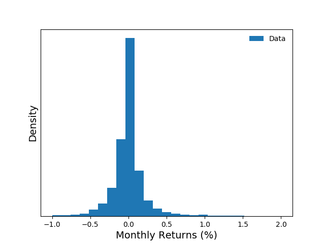
I collected a data set consisting of monthly stock returns from January 31,1980 through January 31, 2017. During this 13,515 day period, there were 5,604,568 quotes from 45,872 stocks.
For each stock, I created a time series of monthly rates of return.
The monthly rate of return, $R_i(t)$, for stock $i$, is computed as
\[ R_i(t) = \frac{\Delta P_i}{P_i(t-1)}, \]
where $\Delta P_i$ is the change in stock price for stock $i$ from
month $t-1$ to $t$ and $P_i(t-1)$ is the previous month's stock
price. The figure below plots a histogram of monthly stock
returns.
Analysis
Now that we have some data in good order we can move onto analysis. In this section, we are going to study the returns by comparing their structure to two parametric distributions. We choose the Gaussian distribution and a less common distribution, the Cauchy distribution. The Cauchy distribution is selected because of its relationship to the Gaussian and because it does not have a mean or a variance.
Gaussian Distribution
To fit a Gaussian distribution to data we need to estimate its mean, $\mu$, and variance, $\sigma^2$. The log-likelihood function of the Gaussian is expressed as \[ \mathcal{L}_{gaussian} (\{x\} | \hat\mu, \hat\sigma^2) = -\frac{n}{2}\log(2\pi) - \frac{n}{2}\log(\hat\sigma^2) - \frac{1}{2\hat\sigma^2} \sum_{i=1}^n(x_i - \hat\mu)^2. \] From this expression, the parameters can be estimated from the data using maximum likelihood. \[ \hat\mu = \frac{1}{n}\sum_i^n x_i = 0.002, \] \[ \hat \sigma^2 = \frac{1}{n}\sum_i^n (x_i - \hat \mu)^2 = 0.056. \]
Cauchy Distribution
The Cauchy distribution is another parametric continuous distribution with similar structure to the Gaussian. However, it has infinite mean and variance. The log-likelihood function for the distribution is expressed as \[ \mathcal{L}_{cauchy} (\{x\} | \hat x_o, \hat\gamma) = -n\log(\hat\gamma\pi) - \sum_{i=1}^n \log \Big(1 + (\frac{x_i-\hat x_o}{\hat\gamma})^2\Big). \]
While maximum likelihood methods can be used to estimate the parameters of the distribution from data, there is a a simpler approach. We compute $x_o$ by taking the median of the data {x}. \[ \hat x_o = \textrm{median} \{x\} = 0.00. \] We estimate $\gamma$ by taking the interquartile range of the data $\{x\}$. \[ \hat\gamma = CDF^{-1} (0.75) - CDF^{-1} (0.25) = 0.068. \]
Likelihood Ratio Test
Now that we have estimated the most likely distributions to have
generated the data, we can compare them to determine
which is a better. Before jumping straight to the test, let's
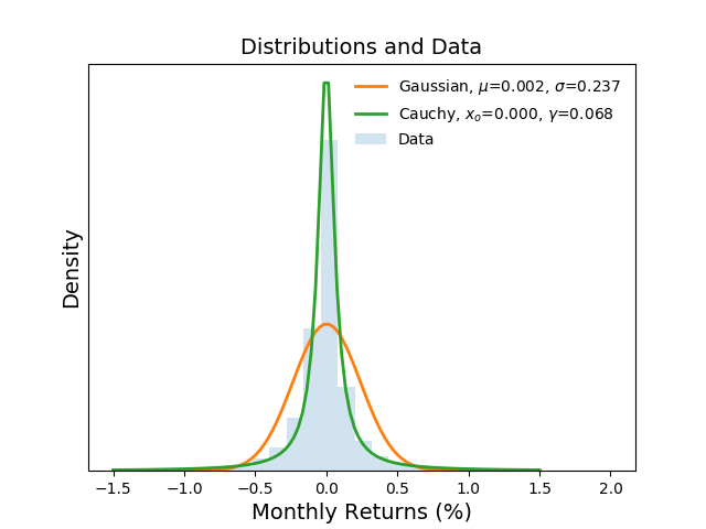
visually inspect the distributions and the data. The following
figure plots the full distributions of the
Gaussian($\hat \mu$, $\hat \sigma^2$) and
Cauchy($\hat x_o$ and $\hat \gamma$) on top the histogram of
empirical data. It is clear to see that the Gaussian distribution
estimates returns to have a wider range of returns with similar
probability while the Cauchy estimates the returns to be in a
narrower range closer to what is observed in the data.
Next, let's inspect the tails of the distributions. The two figures
below show the binned data as well as the estimated probabilities of
return at the left and right extremes respectively.
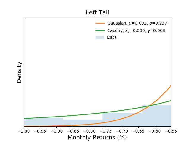
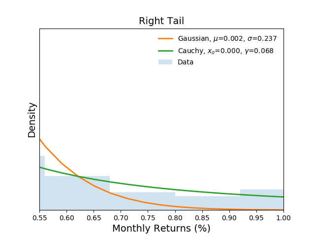
It is clear from the figures that the Gaussian distribution under estimates extreme events while the Cauchy distribution more closely follows the empirical observations.
Now that we have some intuition from the visual analysis, we can a apply more rigorous comparison via a likelihood ratio test. We perform the test by computing the log-likelihood for the Cauchy and Gaussian distributions using the equations noted earlier in the article. Then we take their ratio, \[ \mathcal{R} = \frac{ \mathcal{L}_{cauchy}(\{x\} | \hat x_o, \hat\gamma)} { \mathcal{L}_{gaussian} (\{x\} | \hat\mu, \hat\sigma^2)}. \] If the Cauchy distribution is a better fit to the data we expect to observe a large and positive number. Indeed, the result $\mathcal{R} = 23,525,726.265$, indicates that the Cauchy distribution is a better fit than the Gaussian.
From this result, we can call into question the validity of MPT and CAPM. As previously mentioned, both rely on finite measures of mean and variance and the data clearly show that a parametric distribution with infinite mean and variance fit the data better than a traditional Gaussian distribution. Moreover, if a Gaussian distribution is used to construct a portfolio, we have shown that it will systematically underestimate the extreme risk of a portfolio of domestic equities.
Conclusions
This cursory analysis motivates additional research into not only the statistical properties of market returns but also the generating processes that create such structure [1]. Relatively new research both inside and outside the confines of finance have begun to explore such approaches [2-4].
It is clear that we have much to learn and existing theory, while likely useful in specific instances, does not generalize to represent a unified and complete understanding of how market dynamics produce returns through time.
References
- Bernardo, JM and Bayarri, MJ and Berger, JO and Dawid, AP and Heckerman, D and Smith, AFM and West, M Generative or discriminative? getting the best of both worlds, Bayesian Stat 2007
- Taleb, Nassim Fooled by randomness: The hidden role of chance in life and in the markets Random House Incorporated, 2005
- Farmer, J Doyne and Patelli, Paolo and Zovko, Ilija I The predictive power of zero intelligence in financial markets, Proceedings of the national academy of sciences of the united states of america. 2005
- Galla, Tobias and Farmer, J Doyne Complex dynamics in learning complicated games, Proceedings of the National Academy of Sciences, 2013